A tutorial by AndrewFM
(v1.20)

Introduction

Effekseer is a free, open-source program for making particle effects for games. The effects made with the program can be exported as 2D sprite sheets, AVI files, or as a special proprietary filetype for 3D. The program comes with a unitypackage for using these 3D files in Unity, and also comes with a C++ runtime for using them with DirectX or OpenGL. Effekseer's interface and features have been heavily influenced by BISHAMON, and in a sense Effekseer is just a simpler, less feature rich version of it.

This document is an overview of the program, organized in a fashion similar to a tutorial. It covers many of the features of the program, but it is not an exhaustive manual. However, you can view the original, official Japanese manual for the program here.

The Effekseer project files used to generate the illustrations in this tutorial can be downloaded here.

General Interface

Basically all of the program's features are contained under the 'Window' menu at the top of the screen. Effekseer's layout is fully customizable; any of the windows can be added/removed, resized, repositioned, tabulated, etc... This is all done simply by dragging and dropping them.

Viewer

The Viewer is where you can preview the particle effect you have created. The viewer can be panned with the middle mouse button, can be rotated with the right mouse button, and can be zoomed with the scroll wheel.

The Start and End fields control the time interval that will be previewed when the play button is pressed. These are measured (as is every timing related thing in this program) in frames (60 frames = 1 second). So for example, if you set the interval to [120,180], then when you press the play button it will start two seconds into the animation, and end one second later at the three second mark.

The Step buttons (double arrows) allow you to walk through the animation one frame at a time. The number is the current frame being shown in the viewer.

The grid visibility, color, and other settings can be configured in the program's preferences (Window → Options). Other settings such as background color/image, scene lighting, etc, can also be configured in the preferences.

Node Tree

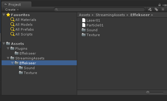
This is the overview of your project's structure, containing all of your particle emitters. Clicking on a node in the tree brings up all of its properties in the various program windows, allowing you to edit anything about it. Right clicking in the node tree brings up a context menu that includes the option to add a new node. The new node will be added as a child of the currently selected node. There is the concept of inheritance in this program (ie: child nodes inherit some properties from their parent nodes), which will be talked about in more detail later. Nodes can also be copy and pasted, which is very useful.

Random Fields

Many numeric fields in the program take on an appearance like the image on the left. These types of fields indicate that they are capable of taking on randomly assigned values. There's two options for input, both of which are functionally equivalent:

Range: You specify a minimum and maximum value, and the assigned value will be any random (real) number that falls between those two extremes.
Gauss: You specify the range instead using a mean and deviation. For example, with {Mean=5, Deviation=2}, the randomly assigned value will fall between 3 and 7.

Particle Emitters (aka, Nodes)

Nodes are the core of this program; they are what actually spawn the particles that make up the particle effects. This section deals with how to modify the ways in which the nodes spawn the particles, but not how to edit the particles themselves. (Editing the behavior and appearances of the particles that have been spawned will be the topic of the proceeding sections)

Basic Settings

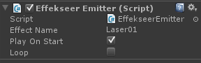
The Basic Settings window contains all of the standard parameters for tweaking the way in which a node spawns its particles. Starting from the top, the Visibility checkmark enables/disables the display of this node's particles in the Viewer. Note this is purely for editing convenience, as the particles will still appear in the final export regardless of the visibility settings.

Name serves no purpose other than your own convenience. Once you start getting many nodes in your node tree, you'll want to give descriptive names to them.

Spawn Count sets the maximum number of particles this node is allowed to spawn. The Infinite checkmark overrides this, and allows the node to spawn particles without limit.

Time to Live sets the lifetime of each spawned particle (in frames). This is local to each particle, and begins counting down as soon as the particle is spawned. Once that duration of time has passed, the particle will automatically be destroyed. This is ignored if Destroy after time is unchecked.

Spawn Rate determines how quickly the node emits particles. A value of 1 means it will spawn one particle per frame. A value of 10 means it will spawn one particle every 10 frames. This can be a decimal number; for example, a value of 0.1 will mean the node will emit 10 particles per frame.

Initial Delay makes the node wait a certain duration of time before emitting its first particle. This is useful for sequential effects where not all of the emitters are immediately active.

Inheritance

As mentioned earlier, inheritance is a feature of this program. If for example, Node A is a parent of Node B, then every single particle that Node A spawns will have an instance of Node B attached to it (so you can have particles that emit other particles). The Basic Settings window has a few parameters I purposely skipped over, that apply to inheritance.

Inherit Position/Rotation/Scale are self-explanitory in what they do, but the drop-down options may be less clear. There are the following three options:

Always: As long as the parent particle exists, this child particle will constantly update its inherited values to match that of the parent particle.
Only on Create: This child particle will inherit the value from the parent particle on spawn, but will then act on its own, ignoring any further updates to the parent particle's values.
Never: The child particle will not inherit the value from the parent particle.

If Destroy with parent is checked, then the particle will be automatically destroyed if the parent particle it was spawned from gets destroyed.

Destroy when no more children is the inverse of the above. If a parent node spawns a finite number of child particles, it will be automatically destroyed as soon as all of those child particles have finished despawning.

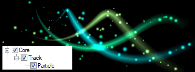
Sample Project "00_Basic/Laser03.efkproj" is a good example of inheritance. Invisible "Core" particles guide the position and rotation of the "Track" particles that inherit them -- this gives the tracks that distinctive zig-zag shape. At the same time, the "Particle" node inherits "Track", using the track's position to allow it to emit tiny particles along the trajectory of the zig-zags.

Spawn Method (Circular)

A separate window from the Basic Settings window is the Spawn Method window. By default, nodes emit their particles relative to a single isolated point in space. There are two other spawn methods, however. The first is Circle.

In Circle spawn mode, particles will be spawned relative to the circumference along a circle. Radius sets the size of that figurative circle.

Init Angle and Final Angle allow you to specify the range over the circle in which to spawn particles. By default this goes from 0 to 360, resulting in particles spawning over the whole circumference. However, this can be reduced to allow spawning only over a specific arc of the circle.

There are a few different modes of spawning along the circle. There is Clockwise and Counter-clockwise, which result in each successive particle spawning in an orderly sequential fashion along the circle (ie: think of clock hands). Random results in each successive particle choosing randomly among any of the available verticies to spawn on.

Verticies control the number of spawning angles the circle supports. For example, if it was 8, then it would take 8 particles in Clockwise/Counter mode to do a full rotation around the circle. Likewise, it if was 8, then there would only be 8 possible angles that Random mode could choose from. If you're using Random mode, you'd probably want to increase the verticies to a high number, like 360, to increase the diversity of the random spawn.

Set angle on spawn has the interesting effect of orienting the Y-axis of each spawned particle to be normal to the surface of the circle at the place where it spawned. The figure below illustrates that functionality.


Particles streched along the Y-Axis, being spawned along a circle.	The effect of enabling "Set angle on spawn" on those particles.

Spawn Method (Spherical)

In many ways, this is very similar to the circular spawn method (except adding a third dimension). Note, however, that sequential spawning does not exist here. It is only possible to spawn particles randomly across the spherical surface.

X Rotation and Y Rotation control the "span" over the sphere's surface in which the particles spawn. By default it is 0, which will not allow any particles to spawn. To have particles spawn over the entire sphere, set the deviation to 180, so you get full 360° rotation over each axis. However, like how you could choose to spawn only along an arc of a circle in the section above, you can utilize localized wedges of the sphere's surface for spawning. See the figures below.


Particles spawned on a sphere, with a full 360° span.	Shrinking rotation to only 60° along each axis. A "spherical wedge".

Particles (Behavior)

Position/Rotation/Scale

The three most important windows for modifying the behavior of emitted particles are the Position, Rotation, and Scale windows. Their names are self-explanitory. The Position windows lets you control how the particles move through space over time. The Rotation window lets you control the orientation and angular velocity of the particles. The Scale window lets you modify the size of the particle over its lifetime.

Each of these windows allows you to choose among different methods of modifying these values over time. By default, the mode is set to Fixed, meaning the emitted particles will take on a static value for that attribute, and stay at that value for the entire duration of its existance. The other modes are explained below.

PVA

PVA stands for Position, Velocity, Acceleration. This is likely the mode you will use most of the time. Position sets the initial values on spawn, Velocity sets the rate of change of the initial values over time, and Acceleration sets the rate of change of the velocity over time.

The default setting of Fixed for position/rotation/scale does not allow you to randomize the initial values. Thus, even disregarding velocity and acceleration, PVA can be used as a randomized variant of Fixed.

Easing

If you know specifically what values the particle will start and end with, Easing is an ideal mode to use. It will gradually transition from the start to the end value over the entire lifetime of the particle.

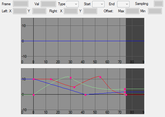
The Ease In and Ease Out dropdown boxes change the style in which the particle transitions between the two values over time. The illustration to the left shows different combinations of easing speeds. The examples respectively refer to the following combinations of {Ease In - Ease Out} pairs:

Slowest-Slowest	Slowest-Normal	Slowest-Fastest
Normal-Slowest	Normal-Normal	Normal-Fastest
Fastest-Slowest	Fastest-Normal	Fastest-Fastest

F-Curve

If Easing and PVA don't do the job, and you need more fine control over how your particle transitions through values over time, F-Curve is the mode you will want to use. The screenshot below shows two F-Curve graphs, the top one showing how the graph initially looks before you touch it, the bottom one showing an example of a graph with values initialized.

The Y-axis of the graph represents value, and the X-axis of the graph represents time. 0 is the time when the particle spawns, and the dark-grey area at the right side of the graph is the time when the particle will die. Like the Viewer, the graphs can be panned with the middle mouse button, and can be zoomed with the scroll wheel. You can also choose the axis of zoom by holding down the Ctrl or Shift button while scrolling the mouse wheel.

To actually add points to the graph, you use the X/Y/Z keys on your keyboard (which intuitively coorespond with the setting of values for the X/Y/Z fields, respectively). Clicking on a point will select it, and you can drag it to reposition it. Dragging straight up or down from a point will create a pivot for a Bezier curve (if the point is set to Bezier mode, which is the default).

Type sets the style of line that connects to and from the selected point. The Linear option will force the lines to be straight, while the Bezier option will allow the lines to be curved.

Max Offset and Min Offset allow you to apply randomization to the F-Curve values. Note that these deviations apply to the whole selected line (ie: it deviates all points on the line by the same random amount), and not to the selected point. It's not possible to randomize on a point-by-point basis.

Start and End also refer to the whole selected line, rather than the currently selected point. They determine the behavior to be taken for defining the values that extend before the first defined point, and after the last defined point. By default they remain at a constant value that matches the first/last point. However, the other options allow you to loop the values over from the beginning. This is particularly useful if the values have a repetitious nature; you then only have to define the first instance of the pattern, and then let the loop fill in the rest for you. The illustration below shows this applied in order to easily make a sine-wave pattern.

Point of Attraction

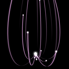
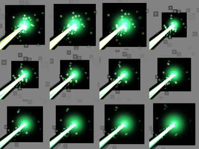
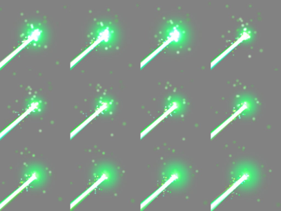
Effekseer allows you define an attraction point for a particle emitter, which acts like a magnet, drawing the spawned particles into it. Sample Project "00_Basic/Homing_Laser01.efkproj", shown below, uses this feature in order to create "homing lasers". They shoot out from a central firing point and home into the attraction point. At the very bottom of the Behavior window, you can define the location of the emitter's Point of Attraction.

By default the point of attraction is not active, so changing its position will not initially have any visible effect. Enabling the attraction point can be done through the Attraction Forces window, by choosing Attraction from the dropdown list.

The Attraction parameter controls how quickly (forcefully) the particles are pulled into the attractor. The Resistance parameter controls how much the particles can resist being pulled directly into the attraction point. For high numbers, the particles will get stuck directly at the point of attraction once being pulled in. For low numbers, the particles will get into an eliptical orbit around the point of attraction (the lower the number, the larger the radius of the orbit). Resistance can also be negative, in which case the point of attraction will actually push the particles away, instead of pulling them in.

Particles (Appearance)

Basic Render Settings

The Basic Render Settings window lets you set some important, general use attributes about a particle's appearance. First and foremost, the Texture field lets you load in any image from your hard-drive to use as the particle's base appearance. Everything else will revolve around altering how this texture gets drawn in the scene.

Blend lets you adjust how the texture responds when other particles overlap with it. The image below shows an example of the different blending types. From left to right: Opacity, Blend, Additive, Subtract, and Multiply.

Filter adjusts the method that's used to resize the particle when it is being scaled. There are only two options... the default, Linear Interpolation attempts to blend the colors of neighboring pixels together. Nearest-Neighbor on the other hand leaves the texture pixelated when it is upscaled.

Fade-In and Fade-Out do exactly as their name implies. The duration specified for these is always relative to the beginning and end of the particle's lifetime. For example, assume Fade-In was set to a duration of 10 frames, and Fade-Out was set to a duration of 20 frames. Then, if the particle was set to live for 100 frames, it would fade in during frames 1-10 after spawning, and would fade out during frames 80-100.

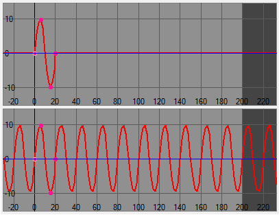
UV lets you draw only a portion of the texture image, rather than the whole thing. This has a variety of uses, and particularly we'll talk about the Scroll and Animation settings:

UV Scroll lets you scroll over the surface of the texture at some fixed X/Y speed. The image to the left shows a smoke texture being UV scrolled over the surface of a conical shape. You'll generally want to make sure that Wrap is set to Repeat, so the texture wraps around as it scrolls.
UV Animation lets you use a sprite sheet as a texture, and play it as an animation. Start should be the coordinate of the top-left of the first frame in the sprite sheet. Size should be the size in pixels of each frame in the animation. X-Count and Y-Count are the number of rows/columns in the sprite sheet that comprise the animation to play. Frame Length is the speed at which the animation will be played.

Distortion allows the texture to be used as a transparent distortion map to affect the appearance of other particles that pass behind it. The brightness of the pixels in the texture affect the areas of distortion. The animations below show this effect in action. Note that it's not the particles that have distortion applied on them, but rather another texture that is sitting in front.


Particles moving back and forth with no distortion.	Those same particles, passing behind a texture with distortion applied.

Sprites

In the Render window, you can choose the method of drawing the texture to the scene. The default method is Sprite, which is where it just draws the texture onto a flat, square surface.

Configuration sets the behavior of the surface, particularly in terms of rotation. By default it is set to Billboard, which means the surface will always automatically rotate to face the camera. This also means it will completely ignore the rotation values set for the particle. The opposite of this is Fixed, in which it uses the particle's rotation values to set the orientation of the surface. The illustration below shows three different configuration settings, applied to particles whose rotation values are assigned randomly. From left to right: Billboard, Fixed (Y-Axis), and Fixed.

Color All blends a solid color over top the entirety of the texture image. Vertex Color on the other hand lets you specify up to four different colors, each cooresponding to a corner of the surface. These colors will blend together by creating a gradient over the surface of the sprite.

Color All offers the ability to randomize the RGBA/HSVA components of the blending color, or offers the ability to gradually ease from one color to another over the lifetime of the particle. You can also use F-Curves for setting the color. This works the same way as the F-Curves for position, except you use the R/G/B/A keys on your keyboard to set waypoints. The F-Curves only offer RGBA mode, and not HSVA mode. However, Hue and Value are fairly easy to replicate using RGB components, as in the images below:

Vertex Coords allow you to edit the relative coordinates of the corner points used by the surface. This allows you to do a few things, the obvious one being to change the shape of the surface to a rectangle, triangle, or other non-square shape. With this you can warp, strech, skew, and crop the texture in various ways. A less obvious use of this is to change the origin of the surface (the point about which the surface rotates and scales). By default the origin point is in the direct center of the surface, but this can be moved by offsetting the values of the vertex coords without actually changing the shape of the surface.

Rings

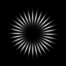
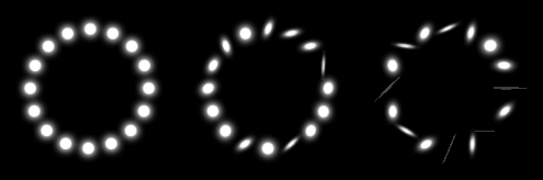
Rings are a powerful option, allowing you to map textures to shapes other than simple flat squares. Despite their name, rings can be used to generate many different geometric shapes, including circles, triangles, cones, cylinders, pyramids, cubes, etc.

Vertex Count allows you to set the number of points that compose the N-sided polygon. By default it is 16, which creates a circular shape (although you can get an even smoother circle by setting it to a higher value like 36). However, this can be set to low values to create other shapes. As seen in the image to the left, 3 vertices creates a triangle, 4 creates a square/diamond, 5 creates a pentagon, etc.

Viewing Angle lets you change the amount of the circle (circumference-wise) to draw... this is very much like the setting used in the circular/spherical spawn methods. The image to the left shows different settings of this value for different shapes. From left to right, it shows 360, 270, and 180 degrees.

Outer and Inner adjust the size/position of the ring's outer and inner radii. With creative settings of these values, you can create a large assortment of shapes. Setting the inner radius to 0, for example, converts the ring to a circle. Additionally, the radius can be adjusted on two different axes, allowing you to have the outer radius be higher up than the inner radius, or vice verse. This allows the creation of 3D shapes, like cones or cylinders. Combining this with the vertex count, you can make even more 3D shapes. For example, a cone with 3 vertices makes a pyramid, and a cylinder with 4 vertices makes a cube.

In terms of color blending, rings support a gradient of up to 3 colors. There's one color for the area closest to the outer radius, one color for the area closest to the inner radius, and a transition color in-between those two. The Center Ratio parameter adjusts the position of the intermediate transition color. A smaller number brings it closer to the inner radius, while a larger number brings it closer to the outer radius.


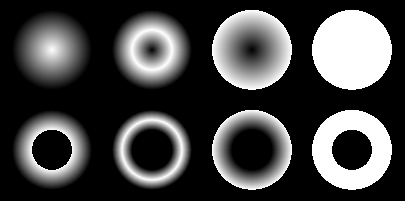
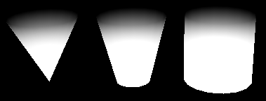
Rings with different opacity, radius, and center ratio settings.	3D shapes made by extending the outer radius in the Y direction.

Ribbons/Tracks

Ribbons allow you to create lines. A few images shown so far in this tutorial have featured ribbons. Particularly, the lines in the Easing animation, and the trails behind the orbs in the "homing missile" example.

They way they work is that each time a ribbon emitter spawns a particle, a line is drawn between it and the previously spawned ribbon segment. By varying the position and velocity of the spawned segments, you can create different shaped line-strips. A common usage of ribbons is to set a ribbon emitter as the child of some other particle, and then have the ribbon emitter's particles inherit the position of the parent on spawn. This will result in a trail being drawn behind the parent particle as it moves.

Tracks are more or less the same as ribbons, except they also incorporate the color features of Rings. A track can define different colors and sizes for the outer, inner, and center points of the line.

Exporting

To 2D Sprite Sheets or Animations

Outputting to a 2D sprite sheet is done through the Recorder window. The X/Y Count determine the layout of the sprite sheet, particularly how many frames each row and column has. Subsequently, this also determines the total number of frames your sprite sheet will contain. For example, {X=4, Y=6} will produce a sprite sheet that has 24 frames, arranged into 4 columns and 6 rows. In addition to exporting as a sprite sheet, you can export directly to a GIF or AVI file, via the format dropdown box.

Start Frame is the frame in the animation the recording should start at. (A small caveat: If you leave this at the default value of 1, your first frame will always be blank. It takes at least one frame for any particles to spawn)

Frame Skip determines the interval at which frames are recorded. For example, if this is set to 2, then only frames {1, 4, 7, 10, ...} will be included in the recording. This is useful for reducing the size of the output, but obviously also results in choppier animations.

Clicking the "Show guide" checkmark will display a black box in the viewer. When exporting to a 2D sprite sheet, the animation will be exported exactly as it it seen within that black box. So you need to make sure to zoom/orient it in the view exactly as you want it to look in the final output.

By default the sprites will export with the black background included. This may make it difficult to use in practice, as you'll always need to use Additive blending to get rid of the background. You can choose "Use original image alpha" from the transparency dropdown to ignore the background, but you have to make sure all the textures you used have transparency/alpha channels of their own. Otherwise, you can try using "Generate alpha" in which Effekseer will automatically try to make the exported sprites transparent for you. (Note that transparency works with the AVI output option as well, so you can easily use the exported AVIs as transparent layers in video editing software)


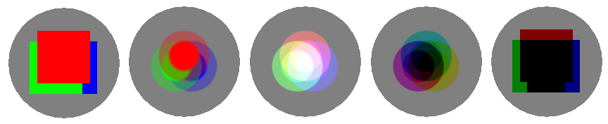
Exported spritesheet without transparency.	Same spritesheet exported using the "Generate alpha" option.

To 3D Effects

File -> Export allows you to export to a *.efk format, which is a proprietary filetype only used by Effekseer. These files can be used by special Effekseer plugins and such to integrate them into your games.

For Unity, the "Effekseer/GameEngine/Unity" folder contains a plugin (for Unity 5) to use the *.efk files in your project. It also contains a sample project showing this plugin in action. After importing the unitypackage, in your project's asset folder, you want to set up the following directory structure:

The exported *.efk files go into the StreamingAssets/Effekseer folder, including any textures the effects use (this is because the textures are not saved in the *.efk file, only references to the textures... thus, the texture files should be named the same, and placed relatively to the *.efk file the same way they were with your original *.efkproj). Then you can add a new Effekseer Emitter to your scene, referencing your effect by name (omitting the efk file extension):